Customer Lifetime Value - Use BG/NBD Model To Simulate Customer Purchase

Dec 1, 2018 • Kyle Yang

American Sign Museum, Cincinnati, OH. Some rights reserved.

Customer Lifetime Value (CLV) is important in today’s business world. There are many articles discussing the calculation of CLV but few involving the simulation of customers’ future purchases.

This article gives the approach to simulate and predict customer behavior with BG/NBD model for the non-contractual and continuous purchase Setting.

This article will not dive into math too much. If you are interested, check this paper and this paper for more about BG/NBD model.

Prerequisite

Language: Python 3

Libraries: Pandas, NumPy, Scipy, Matplotlib, Lifetimes

Data: Online Retail

Data

Libraries

from lifetimes import BetaGeoFitter
from lifetimes.utils import summary_data_from_transaction_data
import pandas as pd
import numpy as np
from scipy import stats
import matplotlib.pyplot as plt
%matplotlib inline

Dataset

df = pd.read_excel("Online Retail.xlsx")
df.head()

Output

	InvoiceNo	StockCode	Description	Quantity	InvoiceDate	UnitPrice	CustomerID	Country
0	536365	85123A	WHITE HANGING HEART T-LIGHT HOLDER	6	2010-12-01 08:26:00	2.55	17850	United Kingdom
1	536365	71053	WHITE METAL LANTERN	6	2010-12-01 08:26:00	3.39	17850	United Kingdom
2	536365	84406B	CREAM CUPID HEARTS COAT HANGER	8	2010-12-01 08:26:00	2.75	17850	United Kingdom
3	536365	84029G	KNITTED UNION FLAG HOT WATER BOTTLE	6	2010-12-01 08:26:00	3.39	17850	United Kingdom
4	536365	84029E	RED WOOLLY HOTTIE WHITE HEART.	6	2010-12-01 08:26:00	3.39	17850	United Kingdom

Get the most recent date of transaction

df['InvoiceDate'] = pd.to_datetime(df['InvoiceDate'])
df['InvoiceDate'].max()

Output

Timestamp('2011-12-09 12:50:00')

Data summary. Here we consider Invoice Date and Customer ID only using BG/NBD model.

data = summary_data_from_transaction_data(df, 'CustomerID', 'InvoiceDate')
data.head()

Output

CustomerID	frequency	recency	T
12346	0	0	325
12347	6	365	367
12348	3	283	358
12349	0	0	18
12350	0	0	310

Implement BG model

bgf = BetaGeoFitter(penalizer_coef=0.0)
bgf.fit(data['frequency'], data['recency'], data['T'])
print(bgf)

Output

<lifetimes.BetaGeoFitter: fitted with 4372 subjects, a: 0.02, alpha: 55.62, b: 0.49, r: 0.84>

Four parameters a, alpha, b and r are generated that can be used to simulate purchases of customers.

Parameters a and b are used for the beta distribution. Parameters alpha and r are used for the gamma distribution.

The use of these two distributions is to simulate the transactions of customers because BG/NBD model, which is the core algorithm to predict CLV and transactions, follow five assumptions:

Purchase count follows a Poisson distribution with rate λ. (While active, the number of transactions made by a customer follows a Poisson process with transaction rate λ.)
Heterogeneity in λ follows a gamma distribution. (Differences in transaction rate between customers follows a gamma distribution with shape r and scale α)
After any transaction, a customer becomes inactive with probability p. (Each customer becomes inactive after each transaction with probability p)
Heterogeneity in p follows a beta distribution. (Differences in p follows a beta distribution with shape parameters a and b)
The transaction rate λ and the dropout probability p vary independently between customers.

BG/NBD model

A class is built for the simulation with given parameters. Assume when observation starts, all customers are alive.

class Simulation:
    def __init__(self, T, r, alpha, a, b, observation_period_end, size):
        self.T = T
        self.r = r
        self.alpha = alpha
        self.a = a
        self.b = b
        self.observation_period_end = pd.to_datetime(observation_period_end)
        self.size = size

    def run(self):
        self.num_alive = self.size
        columns = ['customer_id', 'date']
        self.df = pd.DataFrame(columns=columns)

        if type(self.T) in [float, int]:
            start_date = [self.observation_period_end - pd.Timedelta(self.T - 1, unit='D')] * self.size
            T = self.T * np.ones(self.size)
        else:
            start_date = [self.observation_period_end - pd.Timedelta(T[i] - 1, unit='D') for i in range(self.size)]
            T = np.asarray(self.T)

        probability_of_post_purchase_death = stats.beta.rvs(self.a, self.b, size=self.size)
        lambda_ = stats.gamma.rvs(self.r, scale=1. / self.alpha, size=self.size)

        for i in range(self.size):
            s = start_date[i]
            p = probability_of_post_purchase_death[i]
            l = lambda_[i]
            age = T[i]

            purchases = [[i, s - pd.Timedelta(1, unit='D')]]
            next_purchase_in = stats.expon.rvs(scale=1. / l)
            alive = True

            while next_purchase_in < age and alive:
                purchases.append([i, s + pd.Timedelta(next_purchase_in, unit='D')])
                next_purchase_in += stats.expon.rvs(scale=1. / l)
                alive = np.random.random() > p

            self.df = self.df.append(pd.DataFrame(purchases, columns=columns))
            if not alive:
                self.num_alive -= 1

        self.df = self.df.reset_index(drop=True)
        return self

Class is built for scalability and usability. Different values can be used in parameters for the customized simulation. The artificial transactional data is generated according to the BG/NBD model.

All the details including customer id and timestamp can be found in the simulation result.

Simulate purchases

To simulate the transactions, a random sample of 100 customers are generated.

Any simulation can be built with the given parameters. Here we use the parameters from BG model fitter above and check the transactions detail in next 10 days.

sim = Simulation(T=10, r=0.84, alpha=55.62, a=0.02, b=0.49, observation_period_end='2011-12-20', size=100)
sim.run()
sim.df.head(10)

Output

	customer_id	date
0	0	2011-12-10 00:00:00
1	1	2011-12-10 00:00:00
2	1	2011-12-17 09:44:10.827340800
3	1	2011-12-19 17:57:31.188700800
4	2	2011-12-10 00:00:00
5	3	2011-12-10 00:00:00
6	4	2011-12-10 00:00:00
7	5	2011-12-10 00:00:00
8	6	2011-12-10 00:00:00
9	6	2011-12-17 09:01:58.085731200

We can also simulate the total number of purchases and total number of customers alive expected after any time.

After 10 days

# run simulation multiple times and average results to get total number of customers alive and total number of purchases
sim = Simulation(T=10, r=0.84, alpha=55.62, a=0.02, b=0.49, observation_period_end='2011-12-20', size=100)
simulations_num_alive = []
simulations_num_purchases = []
for _ in range(50):
    sim.run()
    simulations_num_alive.append(sim.num_alive)
    simulations_num_purchases.append(sim.df.shape[0])
print("After 10 days:")
print("Average total number of customers alive:", np.mean(simulations_num_alive))
print("Average total number of purchases:", np.mean(simulations_num_purchases))

Output

After 10 days:
Average total number of customers alive: 99.32
Average total number of purchases: 114.72

After 1 year

sim = Simulation(T=365, r=0.84, alpha=55.62, a=0.02, b=0.49, observation_period_end='2012-12-09', size=100)
simulations_num_alive = []
simulations_num_purchases = []
for _ in range(50):
    sim.run()
    simulations_num_alive.append(sim.num_alive)
    simulations_num_purchases.append(sim.df.shape[0])
print("After 1 year:")
print("Average total number of customers alive:", np.mean(simulations_num_alive))
print("Average total number of purchases:", np.mean(simulations_num_purchases))

Output

After 1 year:
Average total number of customers alive: 94.94
Average total number of purchases: 623.54

You may wonder what if we predict the active customers and transaction after 100 years? It is not possible that there are still many alive users and purchases. This thought is reasonable! The buying habits of customers will not even be the same after 1 year, 1 month or 1 week. This is one of the disadvantages of BG/NBD model you should care about.

Model fitting

Functions from Lifetimes can be used to visualize the prediction and evaluate the model. The algorithm these functions apply are the same as I used above, which is BG/NBD model.

Plot expected vs actual transactions in calibration period

from lifetimes.plotting import plot_period_transactions
plot_period_transactions(bgf)

Outout 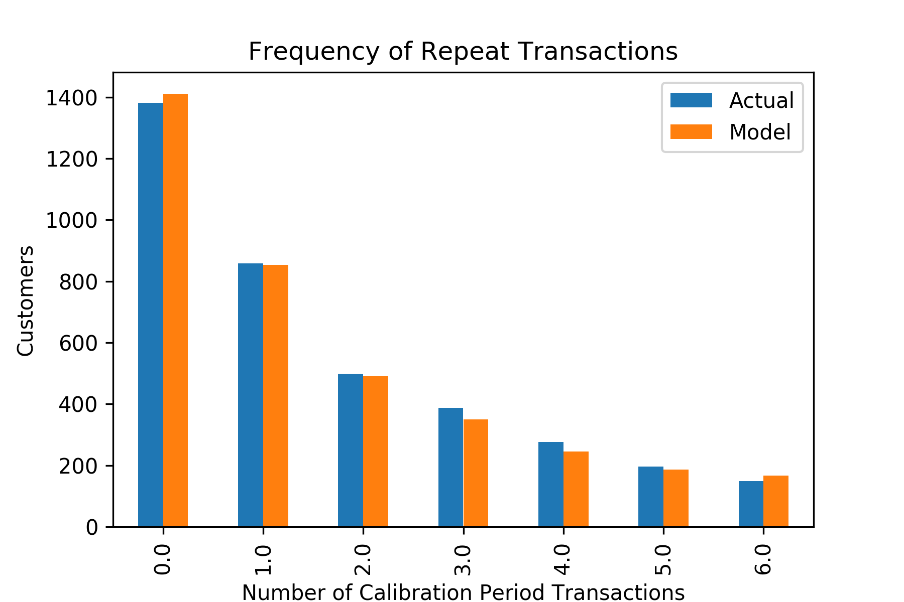model_fit1

Split the dataset and check the plot for purchases in calibration and holdout period

from lifetimes.utils import calibration_and_holdout_data
from lifetimes.plotting import plot_calibration_purchases_vs_holdout_purchases

summary_cal_holdout = calibration_and_holdout_data(df, 'CustomerID', 'InvoiceDate',
                                                   calibration_period_end='2011-06-08', observation_period_end='2011-12-09')

bgf.fit(summary_cal_holdout['frequency_cal'], summary_cal_holdout['recency_cal'], summary_cal_holdout['T_cal'])
plot_calibration_purchases_vs_holdout_purchases(bgf, summary_cal_holdout)

Output 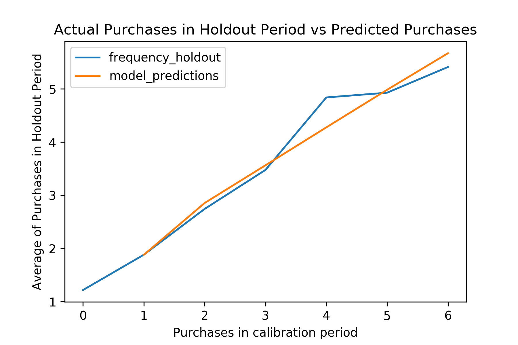model_fit2

Pros and Cons of BG/NBD you should know

The model works well in some ways and poorly in others.

Do well:

The BG/NBD easily lends itself to relevant generalizations, such as the inclusion of demographics or measures of marketing activity.
The model could serve as an appropriate benchmark model.

Do poorly:

The accuracy of the model is usually reflected in the user group level, rather than the level of individual users, and the model of super-complex computing, generalization capability is weak.
The model assumes that the customer is continuously active. This assumption is clearly inconsistent with the reality against the customer life cycle theory that interest about products can change over time.
There could be impacts from covariates, such as marketing activity, that affect the behavior of transactions.