Develop An ARIMA Model With Python

Mojave Desert, CA. Some rights reserved.
This blog shows the steps I take to create the ARIMA model for times series forecasting and how I use Python to implement it with an example.
- Check the characteristics of data
- Find and evaluate the possible models
- Method 1: manual parameter selection
- Method 2: automatic parameter selection
- Choose the better model
- Other things to consider
Check the characteristics of data
Dataset
The dataset I use to create the ARIMA model describes the monthly retail sales for food services and drinking places in the United States from years 1992 to 2018. You can download this dataset here.
Process data
First import packages.
import pandas as pd
import numpy as np
import statsmodels.api as sm
from statsmodels.graphics.tsaplots import plot_acf, plot_pacf
import matplotlib.pyplot as plt
plt.style.use('fivethirtyeight')
%matplotlib inline
Then load and process the data.
data = pd.read_csv("retail_sales.csv")

# convert column DATE to datetime type
data['DATE'] = pd.DatetimeIndex(data['DATE'])

# rename columns
data.columns = ['month', 'sales']
data.head()
Show the first 5 rows of the dataset as below.
| month | sales | |
|---|---|---|
| 0 | 1992-01-01 | 15693 |
| 1 | 1992-02-01 | 15835 |
| 2 | 1992-03-01 | 16848 |
| 3 | 1992-04-01 | 16494 |
| 4 | 1992-05-01 | 17648 |
The data can be plotted as a time series.
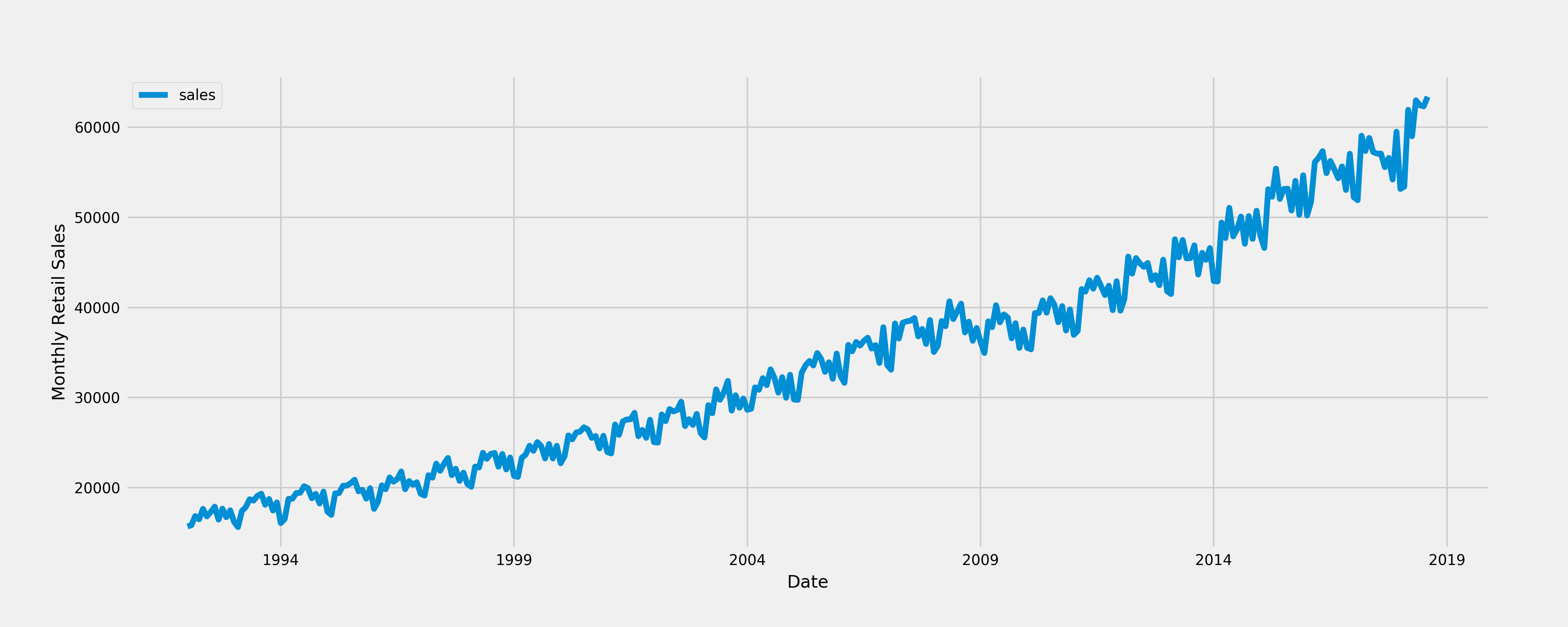
Now we are able to observe the important characteristics of data:
- Trend: there is an upward trend.
- Seasonality: there is a regularly repeating pattern of highs and lows related to certain time of the year. A seasonal difference might be considered.
- Outliers: There is no obvious outliers.
- Variation: It looks like there is increasing variation over time but it is not certain.
For different scenarios,
- If there is seasonality and no trend, then take a difference of lag S.
- If there is linear trend and no obvious seasonality, then take a first difference. A quadratic trend might need a 2nd order difference.
- If there is both trend and seasonality, apply a seasonal difference to the data and then re-evaluate the trend.
Find and evaluate the possible models
Method1 - Manual parameter selection
Differencing
The stationary series is needed when fitting an ARIMA model. If the time series is not stationary, it needs to be so through differencing.
A stationary time series is one whose statistical properties such as mean, variance, autocorrelation, etc. are all constant over time.
Because there is an obvious upward trend with seasonality. We may need to apply a seasonal difference first.
diff = data['sales'].diff(12)
diff = diff.dropna()
diff.plot()
plt.show()
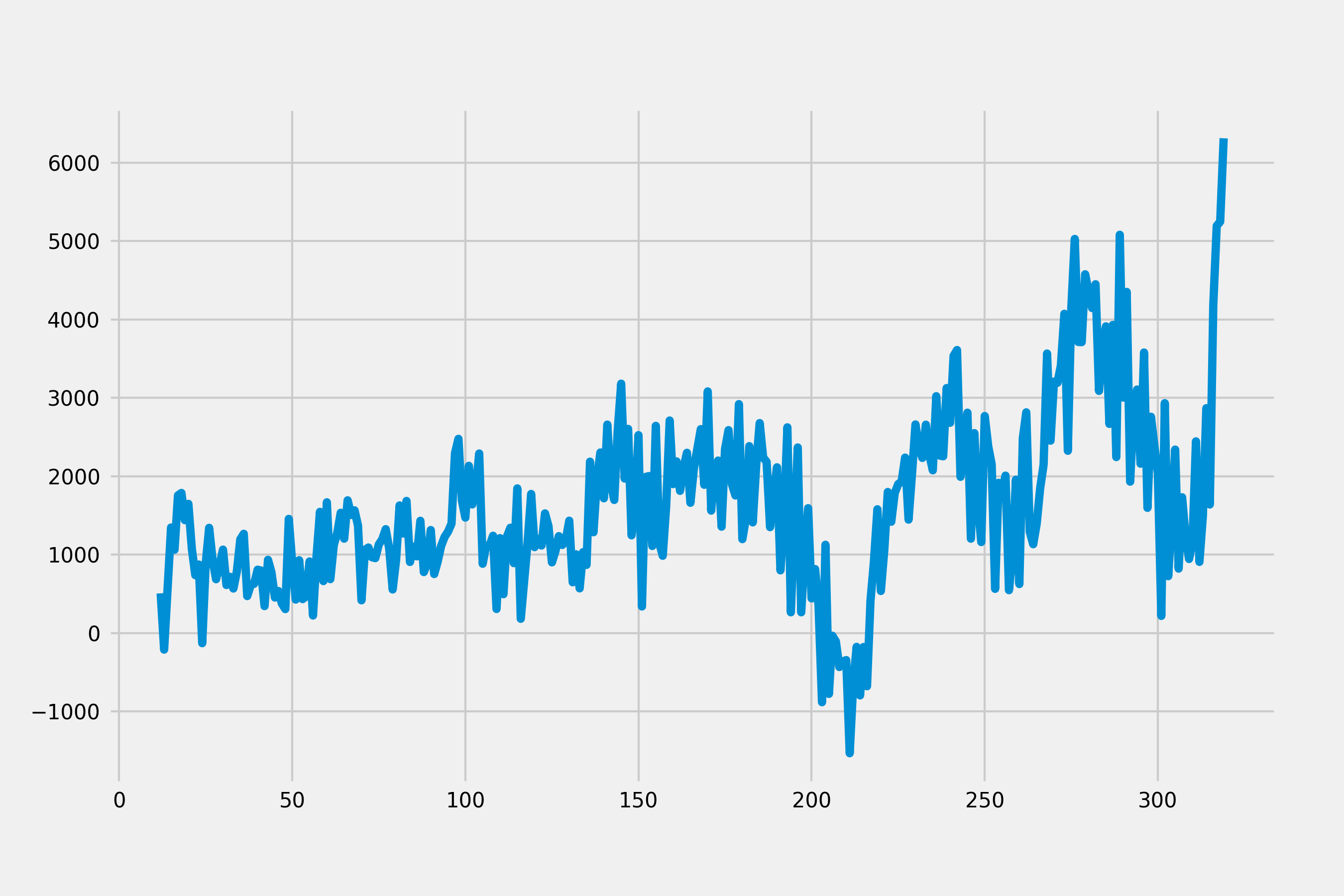
Because trend seems still increasing and the mean of this series varies across different time windows, we could add a non-seasonal difference and check the plot again.
diff = diff.diff(1)
diff = diff.dropna()
diff.plot()
plt.show()
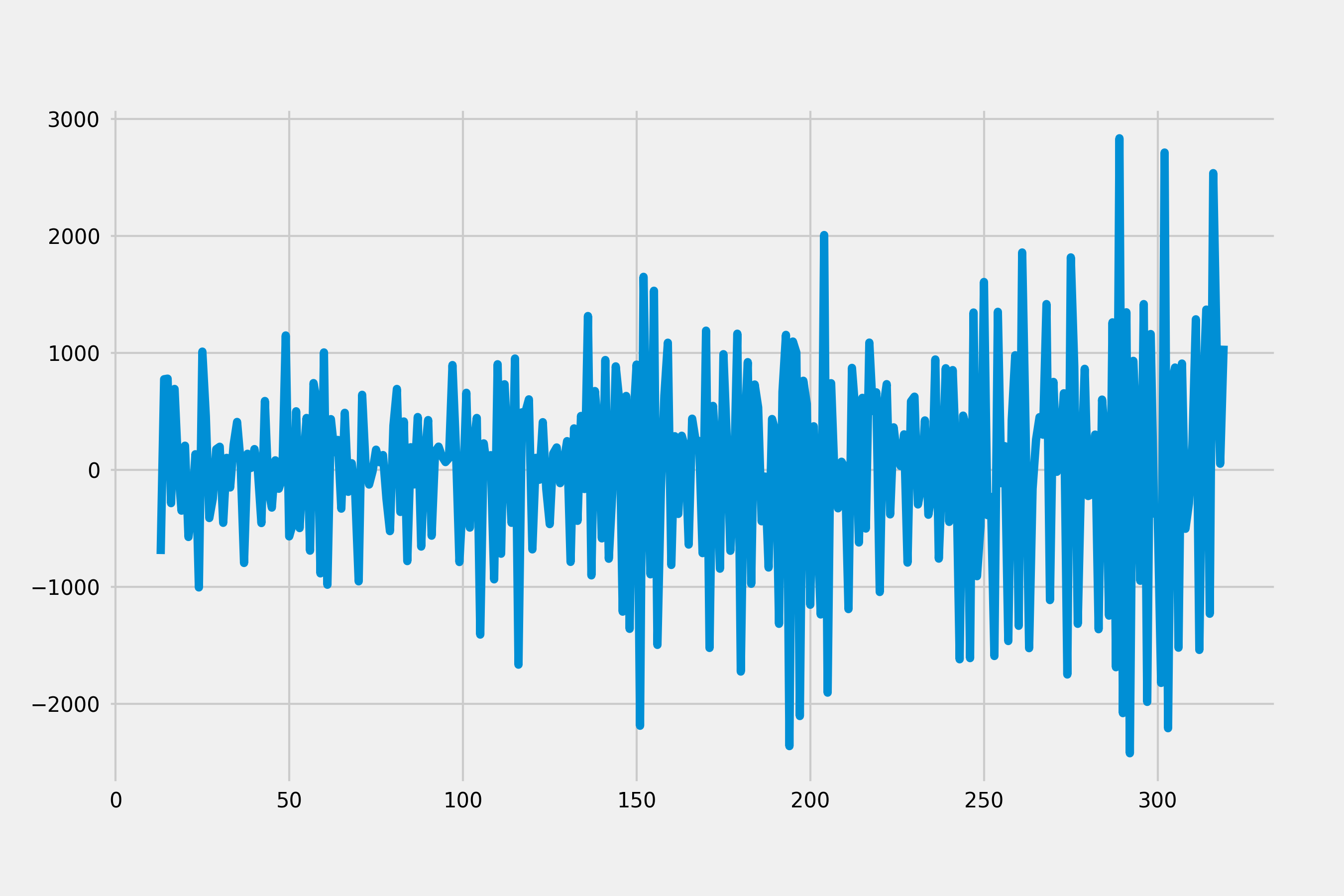
This plot shows a stable series since data values oscillate with a steady variance around the mean of 0. Statistical tests like Dickey-Fuller test can be used to test stationarity of time series.
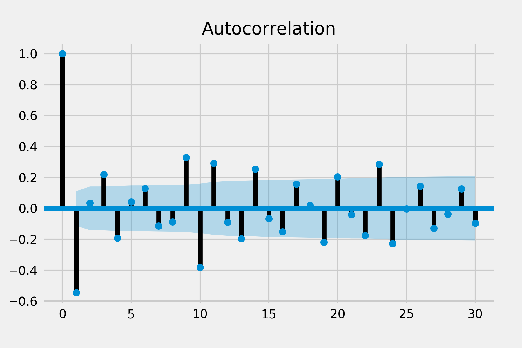
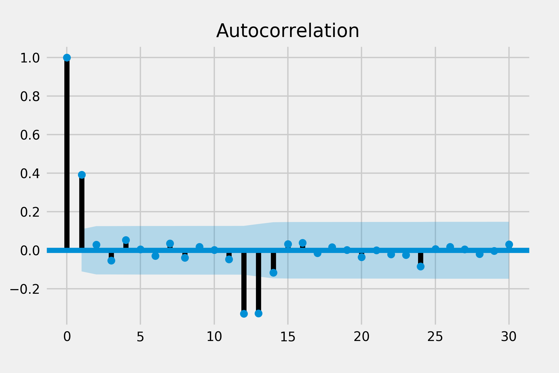
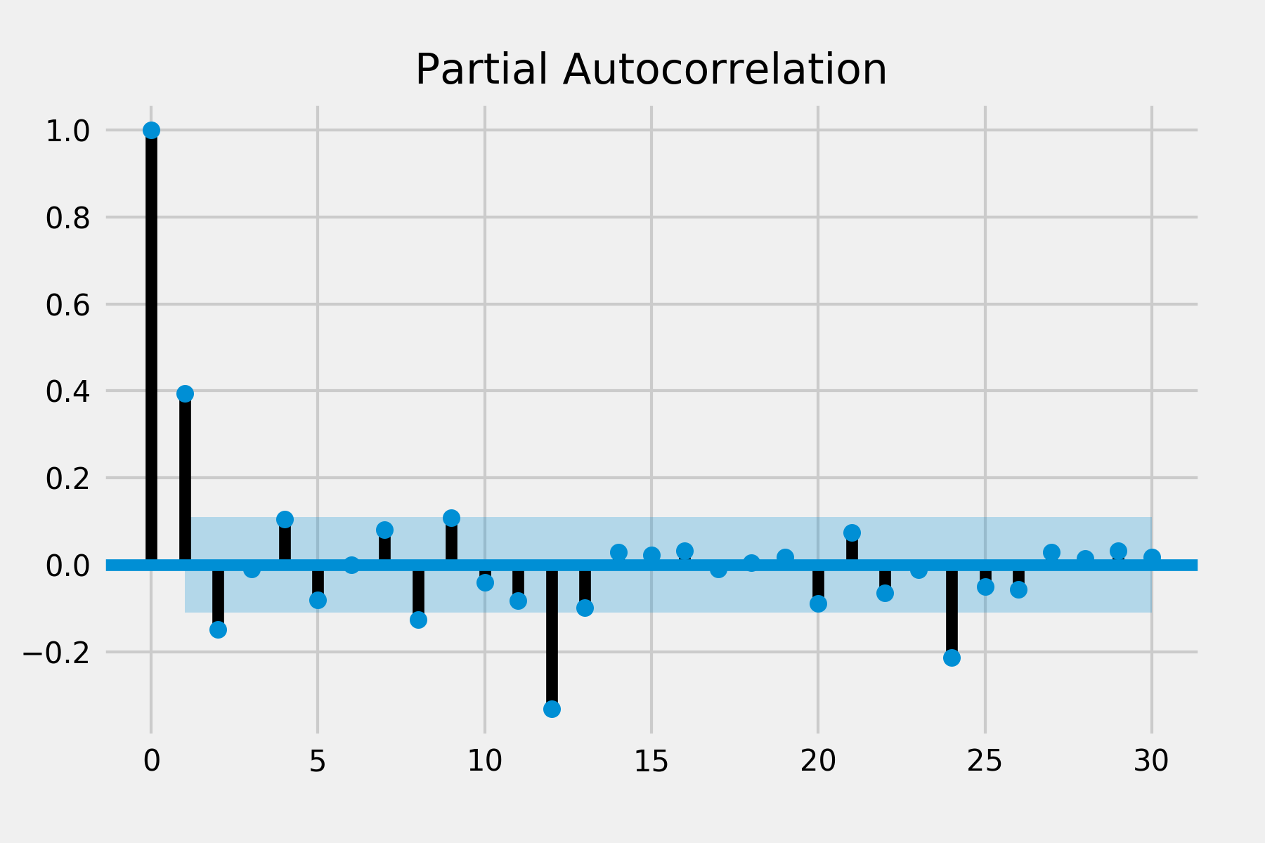
ACF and PACF
plot_acf(diff, lags=30)
plot_pacf(diff, lags=30)
plt.show()
| AR(q) Model | MA(p) Model | |
|---|---|---|
| ACF | Slowly decaying | Only first p autocorrelations are non-zero |
| PACF | Only first q autocorrelations are non-zero | Slowly decaying |
There are significant auto correlations at lag 1 and lag 2 in ACF and there are significant spike of partial auto correlation in lag 1, lag 2 and lag 3 in PACF. There is no obvious spike in other lags so the seasonal pattern may not exist. This suggests that we might use the non-seasonal AR order of 2 and MA order of 3.
Other situation: If all autocorrelations are non-significant, then the series is random. If you have taken first differences and all autocorrelations are non-significant, then the series is called a random walk (Brownian motion) and you are done.
Fitting an ARIMA model
mod = sm.tsa.statespace.SARIMAX(data.set_index('month'),
                                order=(3, 1, 2),
                                seasonal_order=(0, 1, 0, 12),
                                enforce_stationarity=False,
                                enforce_invertibility=False)

results = mod.fit()

print(results.summary().tables[1])
print("AIC:", results.aic)
The output
==============================================================================
                 coef    std err          z      P>|z|      [0.025      0.975]
------------------------------------------------------------------------------
ar.L1         -1.6732      0.051    -32.838      0.000      -1.773      -1.573
ar.L2         -1.5997      0.060    -26.699      0.000      -1.717      -1.482
ar.L3         -0.5174      0.052    -10.015      0.000      -0.619      -0.416
ma.L1          1.1300      0.032     34.951      0.000       1.067       1.193
ma.L2          0.9943      0.053     18.724      0.000       0.890       1.098
sigma2       4.56e+05   4.19e+04     10.887      0.000    3.74e+05    5.38e+05
==============================================================================
AIC: 4802.58755366782
Evaluate and diagnose a possible model
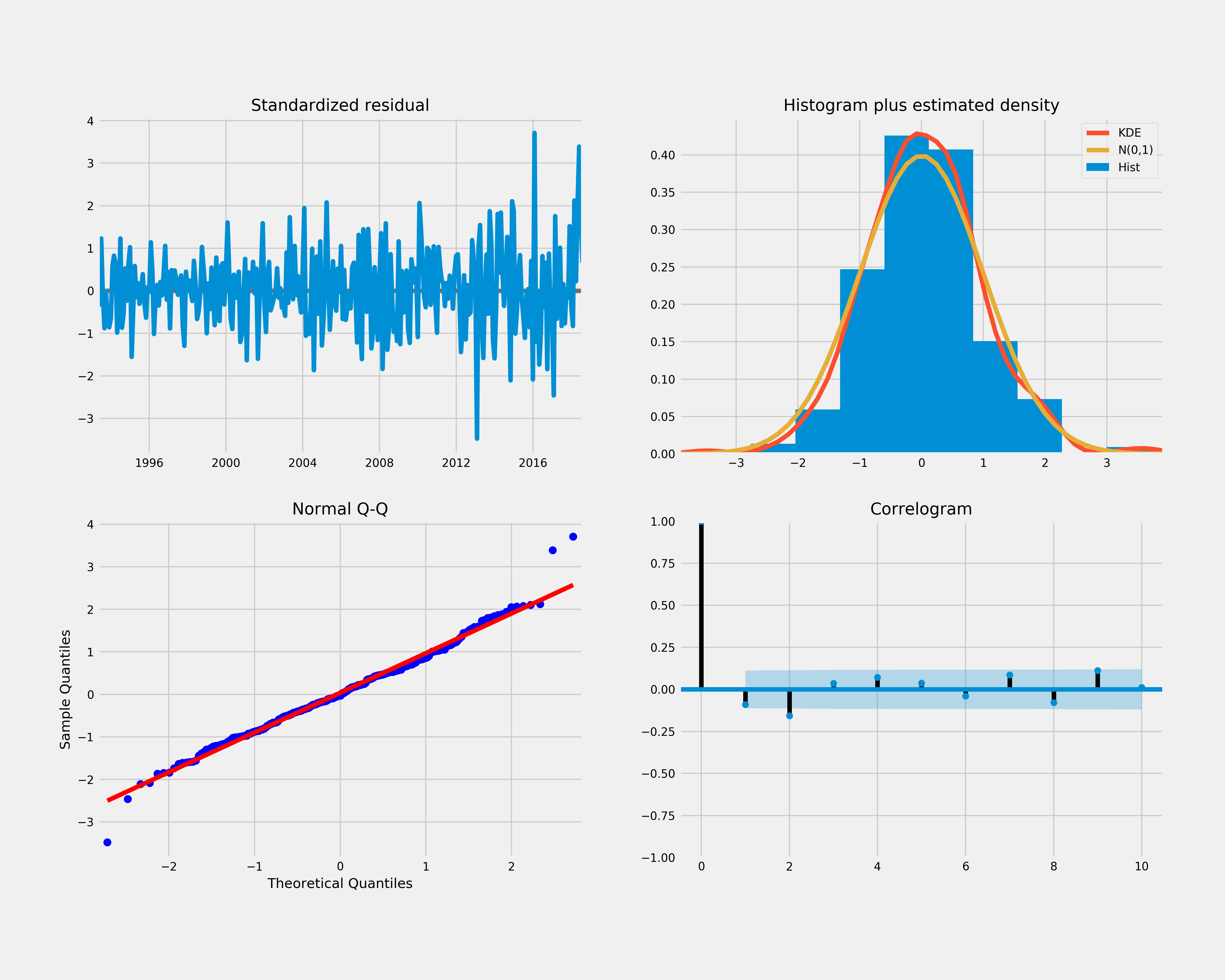
results.plot_diagnostics(figsize=(15, 12))
plt.show()
pred = results.get_prediction(start=pd.to_datetime('2017-01-01'), dynamic=False)
pred_ci = pred.conf_int()

ax = data.set_index('month')['2014':].plot(label='observed', figsize=(20, 15))
pred.predicted_mean.plot(ax=ax, label='forecast', alpha=.7)

ax.fill_between(pred_ci.index,
                pred_ci.iloc[:, 0],
                pred_ci.iloc[:, 1], color='k', alpha=.25)

ax.set_xlabel('Date')
ax.set_ylabel('Sales')
plt.legend()

plt.show()
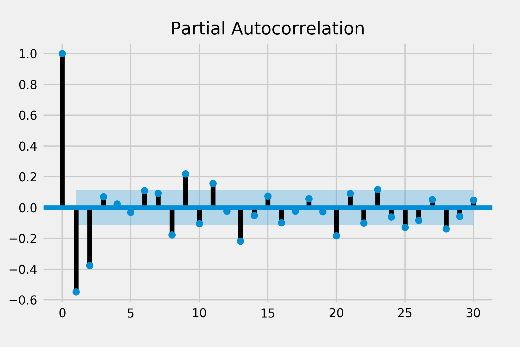
plot_acf(results.resid, lags=30)
plot_pacf(results.resid, lags=30)
plt.show()

- Look at the significance of the coefficients (the table above). All p values of coefficients are 0 that means they are significantly different from 0
- Look at QQ plot (bottom left) and KDE line (top right). It shows the normality of residuals
- Look at the residuals over time plot (top left). It does not display any obvious seasonality
- Look at a plot of residuals versus fits and/or a time series plot of the residuals for constant/non-constant variance
- Look at the ACF of the residuals (bottom right). There are significant spikes at lag 12 and lag 13 in ACF and a spike at lag 12 in PACF so we may try to add seasonal parameters of AR or MA.
The model is not correctly specified, we’ll have to revise our guess by modifying parameters and possibly explain ACF and PACF in a different direction.
mod = sm.tsa.statespace.SARIMAX(data.set_index('month'),
                                order=(3, 1, 2),
                                seasonal_order=(1, 1, 0, 12),
                                enforce_stationarity=False,
                                enforce_invertibility=False)

results = mod.fit()

print(results.summary().tables[1])
print("AIC:", results.aic)
Output is like
==============================================================================
                 coef    std err          z      P>|z|      [0.025      0.975]
------------------------------------------------------------------------------
ar.L1         -1.6801      0.054    -31.068      0.000      -1.786      -1.574
ar.L2         -1.6082      0.063    -25.421      0.000      -1.732      -1.484
ar.L3         -0.5238      0.055     -9.606      0.000      -0.631      -0.417
ma.L1          1.1334      0.027     42.356      0.000       1.081       1.186
ma.L2          0.9920      0.042     23.828      0.000       0.910       1.074
ar.S.L12      -0.2928      0.064     -4.579      0.000      -0.418      -0.167
sigma2       4.56e+05   4.71e-08   9.68e+12      0.000    4.56e+05    4.56e+05
==============================================================================
print("AIC:", results.aic)
AIC score is lower. p values show coefficients are significantly different from 0.
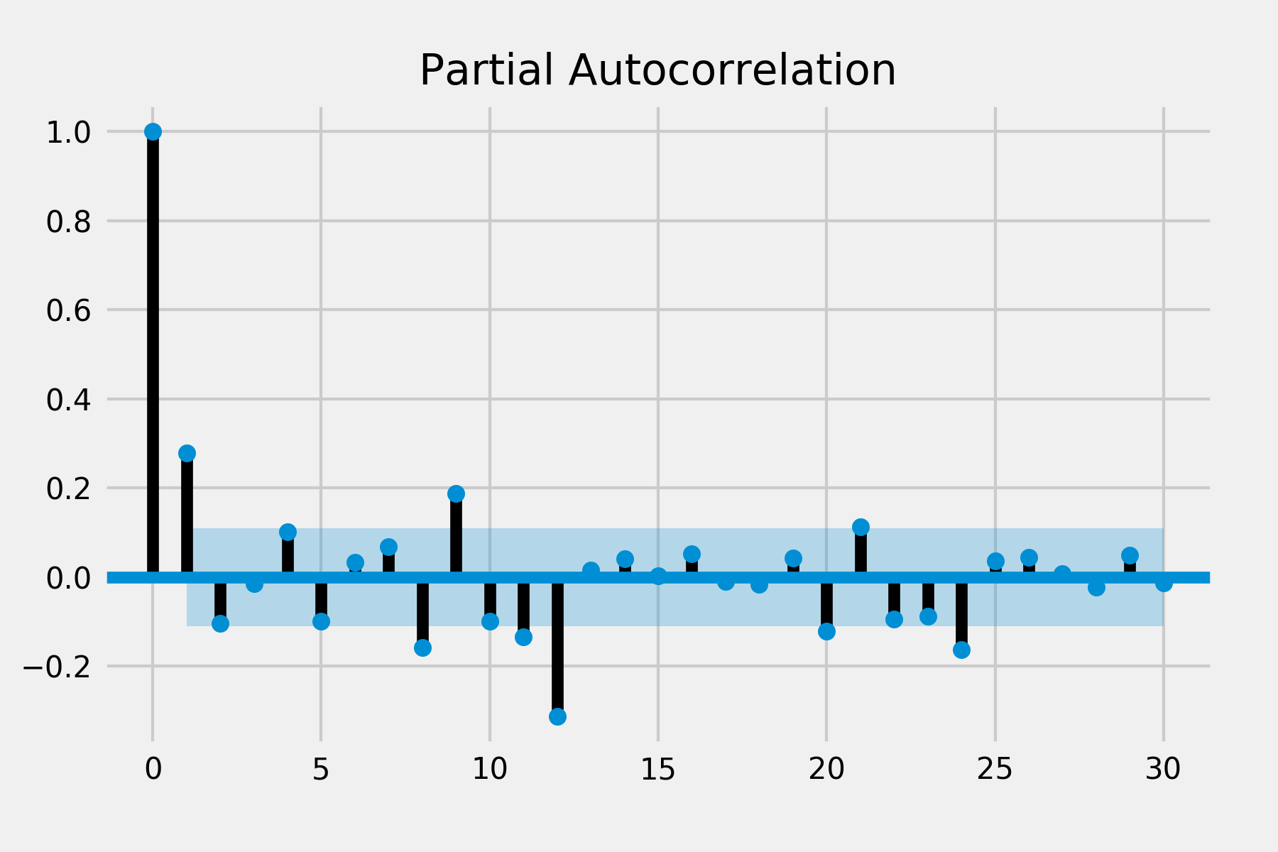
plot_acf(results.resid, lags=30)
plot_pacf(results.resid, lags=30)
plt.show()
PACF looks good but there are still two spikes in ACF. Because it is also difficult to infer p and q from the ACF and PACF, I’ve tried different combinations of seasonal orders. The previous one still provides a better result and reasonable parameters to interpret.
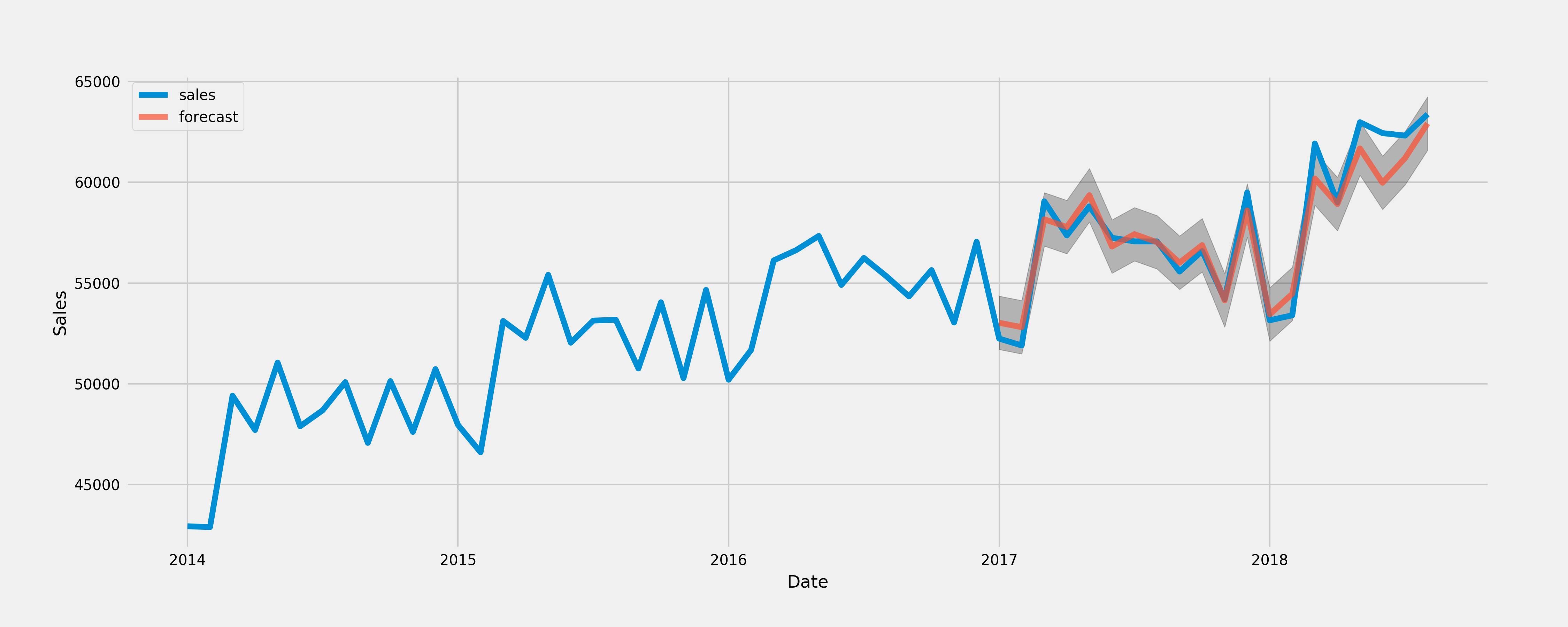
Validate the model
pred = results.get_prediction(start=pd.to_datetime('2017-01-01'), dynamic=False)
pred_ci = pred.conf_int()

ax = data.set_index('month')['2014':].plot(label='observed', figsize=(20, 15))
pred.predicted_mean.plot(ax=ax, label='forecast', alpha=.7)

ax.fill_between(pred_ci.index,
                pred_ci.iloc[:, 0],
                pred_ci.iloc[:, 1], color='k', alpha=.25)

ax.set_xlabel('Date')
ax.set_ylabel('Sales')
plt.legend()

plt.show()
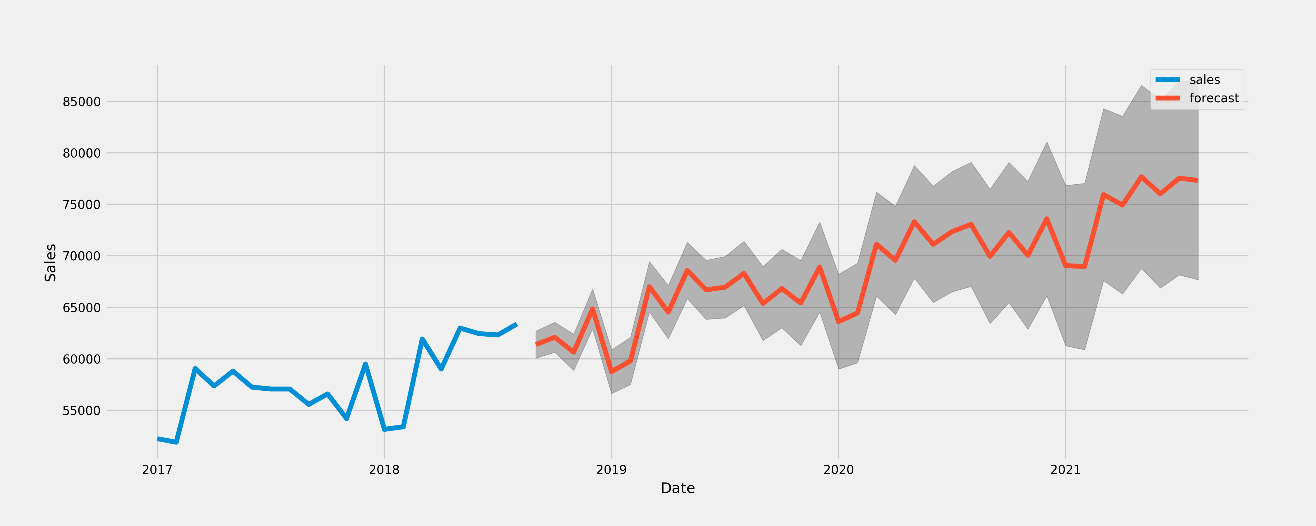
Make forecasting
pred_uc = results.get_forecast(steps=36)
pred_ci = pred_uc.conf_int()

ax = data.set_index('month')['2017':].plot(label='observed', figsize=(20, 15))
pred_uc.predicted_mean.plot(ax=ax, label='forecast')
ax.fill_between(pred_ci.index,
                pred_ci.iloc[:, 0],
                pred_ci.iloc[:, 1], color='k', alpha=.25)

ax.set_xlabel('Date')
ax.set_ylabel('Sales')

plt.legend()
plt.show()
Method2 - Automatic parameter selection
Try different combination of parameters (pretty similar to grid search for machine learning process) to find the optimal selection of parameters by checking AIC/BIC score.
Create non-seasonal and seasonal parameters
# non-seasonal order
p = d = q = range(0, 4)
pdq = list(itertools.product(p, d, q))

# seasonal order
p = d = q = range(0, 2)
s = [12]
seasonal_pdq = list(itertools.product(p, d, q, s))
Fit the ARIMA model using different combination of parameters
for param in pdq:
    for param_seasonal in seasonal_pdq:
        try:
            mod = sm.tsa.statespace.SARIMAX(data.set_index('month'),
                                            order=param,
                                            seasonal_order=param_seasonal,
                                            enforce_stationarity=False,
                                            enforce_invertibility=False)

            results = mod.fit()

            print('ARIMA{}x{}12 - AIC:{}'.format(param, param_seasonal, results.aic))
        except:
            continue
The outputs is like
ARIMA(0, 0, 0)x(0, 0, 0, 12)12 - AIC:7601.915487380611
ARIMA(0, 0, 0)x(0, 0, 1, 12)12 - AIC:7333.604715990744
ARIMA(0, 0, 0)x(0, 1, 0, 12)12 - AIC:5534.639806455742
ARIMA(0, 0, 0)x(0, 1, 1, 12)12 - AIC:5208.000484472617
ARIMA(0, 0, 0)x(1, 0, 0, 12)12 - AIC:5120.972151463306
ARIMA(0, 0, 0)x(1, 0, 1, 12)12 - AIC:5105.101105479268
ARIMA(0, 0, 0)x(1, 1, 0, 12)12 - AIC:5056.488492581053
ARIMA(0, 0, 0)x(1, 1, 1, 12)12 - AIC:5038.368220316868
ARIMA(0, 0, 1)x(0, 0, 0, 12)12 - AIC:7349.690332433109
ARIMA(0, 0, 1)x(0, 0, 1, 12)12 - AIC:12485.014390547416
ARIMA(0, 0, 1)x(0, 1, 0, 12)12 - AIC:5304.233349330357
...
Find the parameters that has the lowest AIC. Then evaluate and diagnose the model following the final step of method1.
Select the better model
If there are multiple models that are possibly a good fit, we can choose the multiple considering other factors.
- Possibly choose the model with the fewest parameters.
- Examine the estimate of the variance. Pick the model with the generally lowest standard errors for predictions of the future.
- Compare models with regard to statistics such as the MSE (the estimate of the variance of the wt), AIC, AICc, and SIC (also called BIC). Lower values of these statistics are desirable.
Other things to consider
If there is a changing, possibly volatile variance, consider using ARCH (autoregressive conditionally heteroscedastic)/GARCH (generalized autoregressive conditional heteroskedasticity).
If the time series is multivariate, VAR (Vector autoregressive) and ARIMAX (Autoregressive Integrated Moving Average with ExplanatoryVariable) model could be the choice.